Coastal Vulnerability Index
The index integrates six physical variables in a quantifiable way to reflect the coast’s relative vulnerability to physical changes caused by sea-level rise. This method produces numerical data that cannot be immediately correlated to specific physical effects. However, it does emphasize the areas where the various effects of sea-level rise may be the most severe.
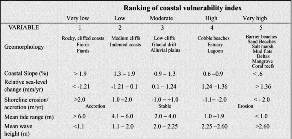
Ranking of the coastal vulnerability index variables
Once each section of coastline is assigned a risk value for each specific data variable, the coastal vulnerability index is calculated as the square root of the geometric mean of these values divided by the total number of variables.
Data Download
The data was downloaded from different platforms which included the Google Earth Engine platform, Global lithological dataset and the Ecological coastal units site based on the variable in question.
Data Processing Steps
Geomorphology
The Geomophological dataset was downloaded from the global lithological portal given below; Global lithological dataset.
It was then subset to the generated study area map of the North Africa region. On the layer styling panel, symbolize the data into 5 classes using the discrete interpolation and then use the interpolation output to classify the data into five classes to give them the degree of erosivity using the qgis reclassify by table tool as shown the the figure below;
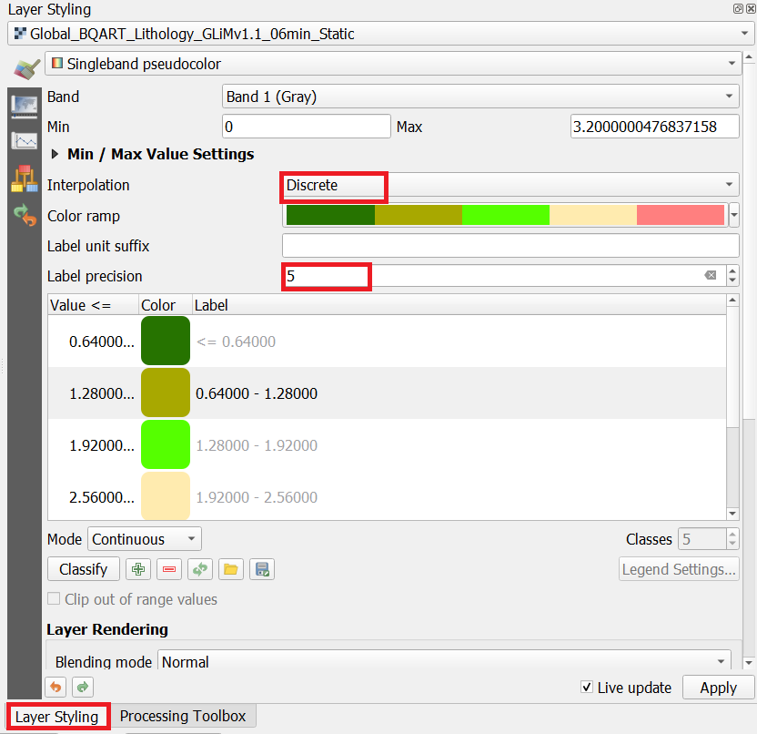
Layer Styling
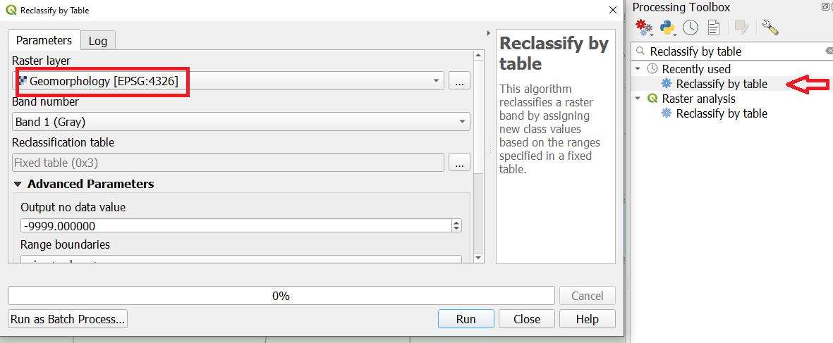
Geomophology reclassify by table
The result of the re-classification should be 5 classes with a risk value of 5 classes whereby value 1 is very low and value 5 is very high.
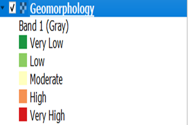
Geomophology Erosivity Classes
Upload to MISLAND Service
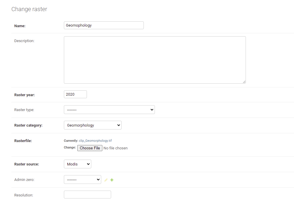
Uploading the data to MISLAND service
Coastal Slope
Download the elevation raster file from Google Earth Engine Subset to the North Africa coastal region using the region’s shapefile. To compute slope, Open Qgis > Raster > Analysis > Slope. The slope computation window opens as shown below:
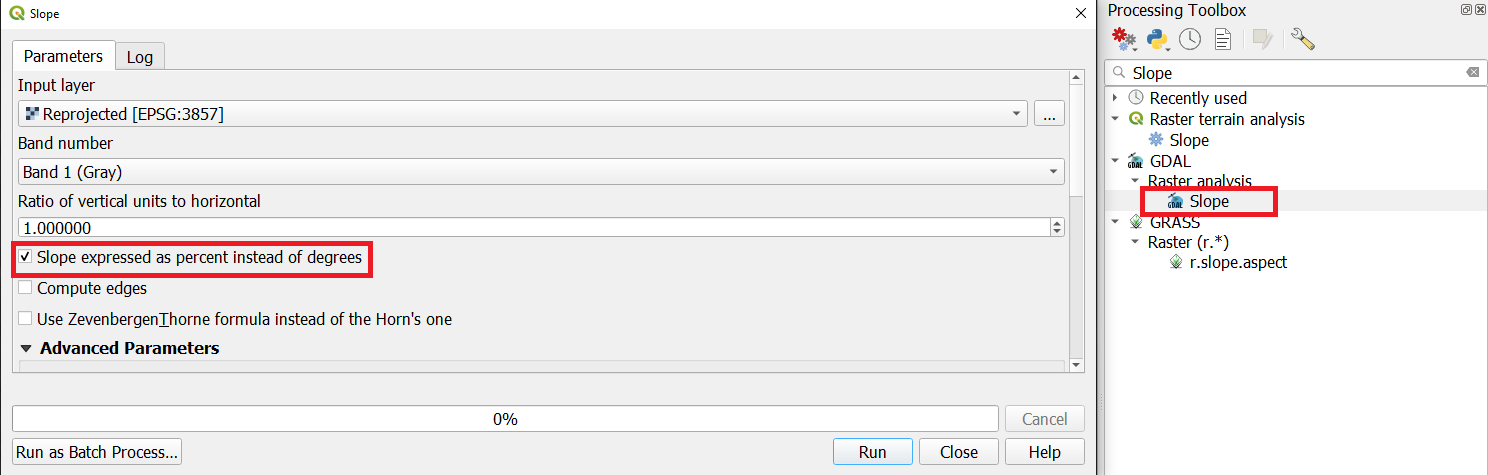
Slope Computation
After a successful slope computation, symbolize the it using the discrete interpolation method in Qgis software and then reclassify it into five classes using the Qgis reclassify by table tool.
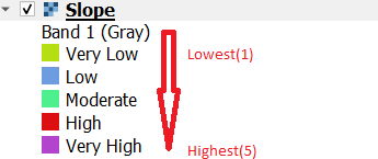
Slope ranked classes
Note
The class ranges should be obtained from the layer styling value label whereby the lowest is assigned value 1 whereas the highest is assigned value 5.
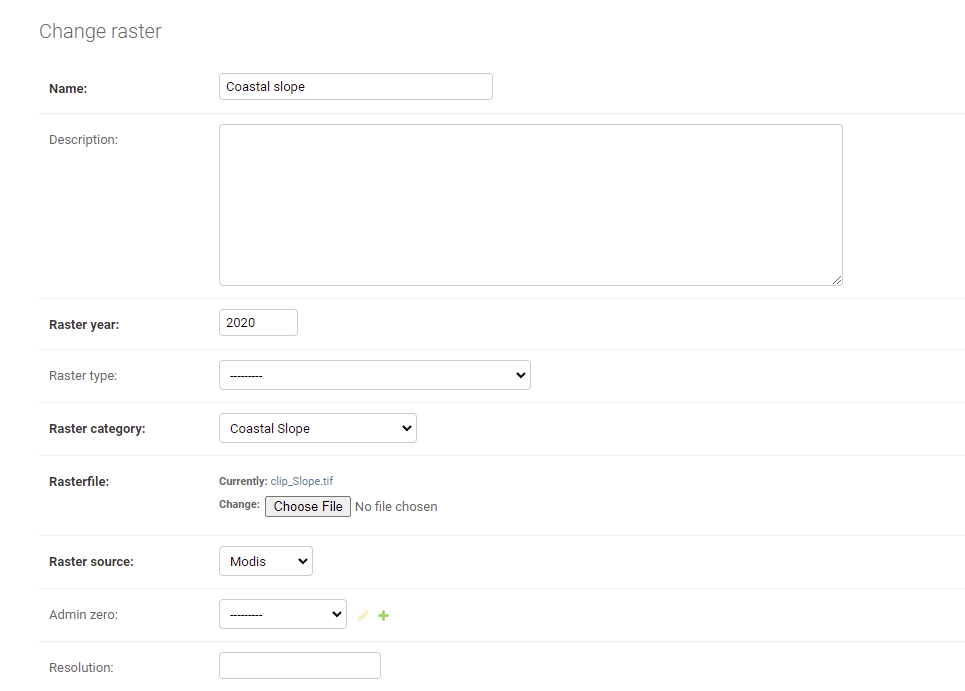
Uploading the data to MISLAND service
Tidal Range
Download the data from the Coastal Ecological Units (ECU) The data comes as a shapefile with different data attributes of 10 variables. First convert the data into a raster using the Rasterize GDAL tool in Qgis. Remember to change the burn-in field value to TIDAL RANGE. Leave the other options as default and click run.
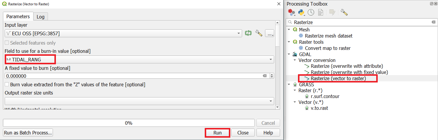
Tidal Range Raster Conversion
Next is to reclassify the data and assign the class ranges as it was done in the Geomophology data preparation.
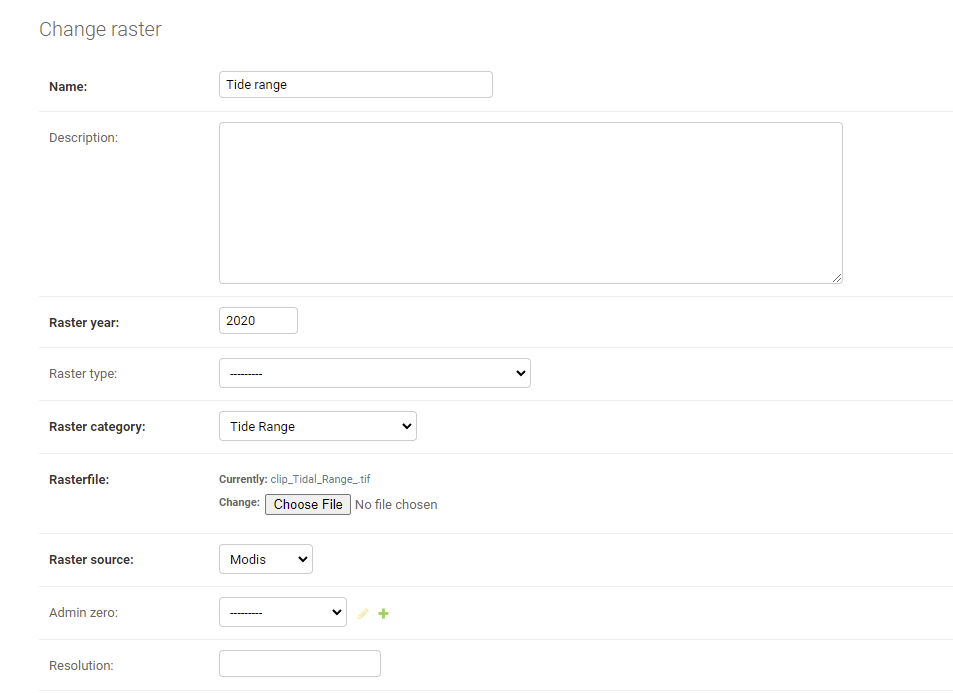
Uploading the data to MISLAND service
Wave Height
Download the data from global wave statistics, and subset it to the North Africa coast region. Follow the same procedure as the one used in the Geomophology data preparation. to classify the data and rank into into 5 categorical classes.
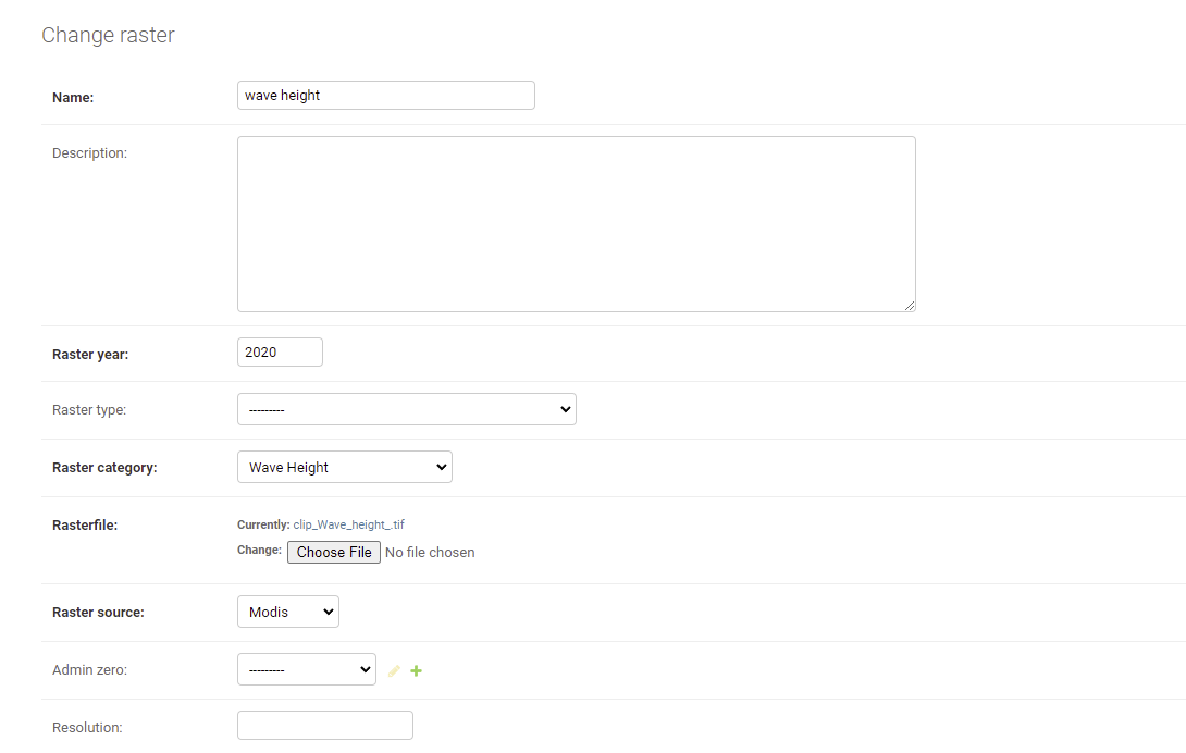
Uploading the data to MISLAND service
Shoreline Erosion
Download the data from the Coastal Ecological Units (ECU) and then follow the procedure as the one given in Tidal Range data preparation.
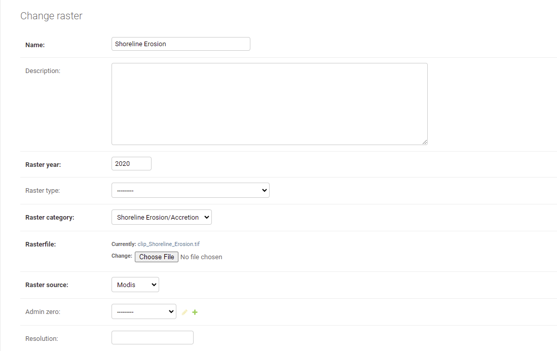
Uploading the data to MISLAND service
Sea Level Rise
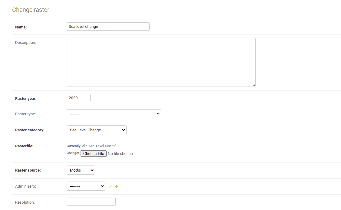
Uploading the data to MISLAND service